DF-11 MRI Performance Test Phantom, Comprehensive MRI QA Phantom
Mode:DF-11
Type:QA-Phantom
Contact: ken@hkmedqc.com
DF-11 MRI Performance Test Phantom, Comprehensive MRI QA Phantom.pdf

Phantom Components
Slice Thickness Ramps
The slice thickness ramps are mounted on the exterior of the test cube. Each ramp is 2 mm thick and 10 mm wide, positioned at a 14° angle relative to the phantom coordinate axes, providing a magnification factor of 4 for slice width measurement. Opposite ramp pairs intersect at the center of the test cube for positioning and calibration.
Spatial Resolution Test Cards
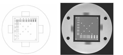
There are three sets of spatial resolution test cards, allowing resolution testing in the coronal, axial, and sagittal planes. Each set is made of 2 mm thick acrylic plates supported by channels inside the test cube. The test is performed using a series of rectangular slots, covering the following line pairs: 2, 2.5, 2.7, 3, 4, 5, 6, 7, 8, 9, 10, 11 Lp/cm. One of the test cards has 3 mm holes arranged in squares of 2 cm, 4 cm, and 8 cm spacing for geometric distortion testing.
Sensitivity Vials
Sensitivity samples are stored in four cylindrical vials with outer diameter 1.9 cm and inner diameter 1.6 cm. The vials can be filled with various solutions through 0.6 cm ports on the outside of the cube for T1 and T2 measurements.
Cube Support Plates
Two cube support plates fix the cube inside the cylinder, allowing easy installation and removal. While positioning the cube, the support plates also provide information for spatial linearity measurements. The support plates have 3 mm holes centered on squares of 8 cm, 10 cm, and 12 cm, with the phantom axis as the center. At the corners of the larger squares, there are four sets of 2 cm squares. This design allows measurement of both global and local geometric distortion.
Low Contrast Module
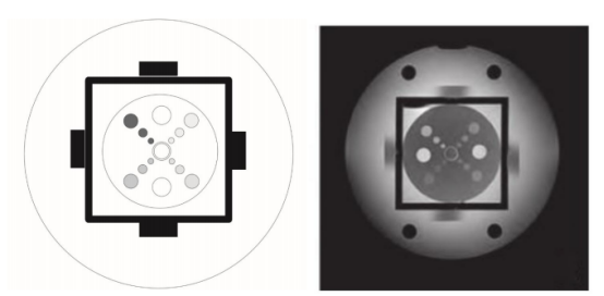
The low contrast test module consists of an acrylic disc mounted on the base of the test cube. Four groups of three circular grooves have depths of 0.5 mm, 0.75 mm, 1.0 mm, and 2.0 mm, and diameters of 4 mm, 6 mm, and 10 mm (from the center outward).
Housing
The housing assembly includes the outer shell and cube support plates (supporting the 10 cm test cube). The top disc of the housing is removable and includes an artifact test module. When the test cube and support plates are removed, the housing can be used for comprehensive spatial uniformity measurements. The housing is easy to clean and allows the use of gels and liquid solutions; multiple ports allow unrestricted flow during drainage.
1. Operating Instructions
1.1 Pre‑scan Preparation
During storage and transportation, air bubbles may adhere to internal test components. Remove as many bubbles as possible so that all imaging test planes are unaffected before scanning.
1.2 Phantom Positioning
Place the phantom stably on the head coil base of the patient table. Use a spirit level to adjust the phantom horizontally in two perpendicular directions, and correctly install the receive coil. Use the laser positioning system to determine the phantom center, then move the phantom to the magnet isocenter. Register the scan information and set the scanning parameters.
1.3 Phantom Scanning
First perform a three‑plane localizer scan. If the phantom is correctly positioned, the short lines on both sides of the square will be equal in length, horizontally level, and symmetrically distributed. If not aligned, perform a second localizer scan – the scan angle can be adjusted, otherwise reposition the phantom. Next, on the qualified localizer image, acquire axial scans of the various test planes as shown in the figure below.
1.4 Signal‑to‑Noise Ratio (SNR) Measurement
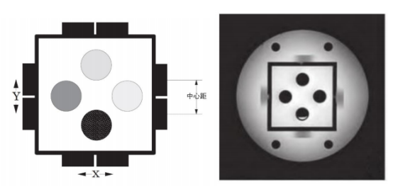
In the center of the image shown in Figure 1, draw a large circular region of interest (ROI) and record its signal intensity (Sinner) and noise (SDinner). Draw four small circular ROIs (area ~200 mm² each) at the four corners outside the phantom, and record the average background signal intensity (Souter). Calculate SNR using formula (1):
Note: If obvious artifacts are present within the ROI, SNR measurement should not be performed.
1.5 Image Uniformity Measurement
In the square image of Figure 1, uniformly select 9 ROIs, each with an area of approximately 200 mm². Record the signal intensity S of each ROI and calculate the image uniformity using the following formula:
1.6 Spatial Resolution
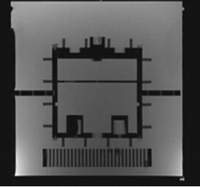
In Figure 2, reduce the window width to its minimum, adjust the window level to obtain the sharpest display of image details, and visually determine the maximum number of line pairs that can be clearly resolved – that is the spatial resolution.
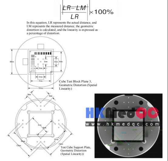
1.7 Geometric Distortion Test
The phantom includes two test modules for geometric distortion: one on the spatial resolution test card and one on the cube support plate (see Figure 3). Measure the distances between holes in the frequency‑encoding direction (X) and the phase‑encoding direction (Y), compare with the true distances (indicated in Figure 3), and substitute into the following formula:
where LR is the real distance and LM is the measured distance. Linearity is expressed as percent distortion.
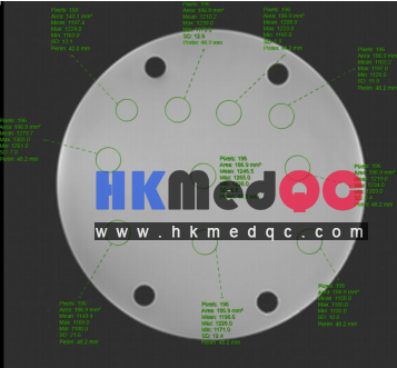
1.8 Low‑Contrast Resolution
In Figure 4, simultaneously adjust window width and level to obtain the clearest image details. Visually determine the smallest depth and smallest diameter of the holes that can be clearly resolved – that is the low‑contrast resolution.
The low‑contrast test card has holes with the following diameters and depths:
- Hole diameters: 4.0 mm, 6.0 mm, 10.0 mm
- Hole depths: 0.5 mm, 0.75 mm, 1.0 mm, 2.0 mm
To determine the actual contrast value, calculate the average of several measurements from the low‑contrast section.
1.9 Slice Thickness Measurement
On the four test planes of the cube, there are two pairs of opposing 14° ramps: one pair oriented along the X‑axis, the other along the Y‑axis. The ramps are made of 2 mm thick, 10 mm wide acrylic strips positioned at a 14° angle to the imaging plane. These ramps are used to estimate slice width. (To determine the full width at half maximum of the gradient from the scan image, identify the gradient peak and background values.)
First, near each of the four ramp images in Figure 5, select an ROI of area 200 mm². Record the signal intensity of each ROI as S1, S2, S3, S4. Then set the window width to 1 and adjust the window level until each ramp image just disappears. The window level at that point is the maximum value of the ramp image: L1, L2, L3, L4.
Set the four window levels to (S1+L1)/2, (S2+L2)/2, (S3+L3)/2, (S4+L4)/2 respectively. Measure the width of each ramp image and calculate the average to obtain the full width at half maximum (FWHM).
Slice thickness (mm) = FWHMY × 0.25